Training a YOLOv5 Model for Face Mask Detection

Introduction

In the previous article of this series, we labeled a face mask dataset. Now is the time for the most exciting part of this project – the model training.

Preparing the Training and Validation Data

Just like any other model, YOLOv5 needs some validation data to determine how good the inferences are during and after training. This is why we need to split our set of images into train and val datasets with their corresponding .txt files. Usually, the split ratio is 80% for training to 20% for validation, and these must be distributed as follows:

Dataset
|
| -- images
|      | -- train
|      | -- val
|
| -- labels
|      | -- train
|      | -- val
|
| -- dataset.yaml

I split the data manually; I placed the first 3,829 images in the images/train directory, and the remaining 955 in the images/val one. I then copied their corresponding .txt files to labels/train and labels/val, accordingly.

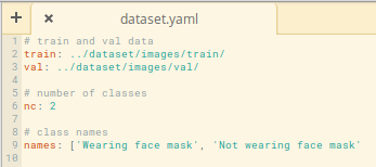
The dataset.yaml file tells the model how the dataset is distributed, how many classes there are, and what their names are. This is how the file looks in our case:

The functions are:

• Line 1 indicates the relative path for the train images set
• Line 2 indicates the relative path for the validation set
• Line 6 states how many classes the dataset contains
• Line 9 defines the names for each class

Every time you train a YOLOv5 model you’ll have to create this file manually. Luckily, it’s not a complex task.

Training the YOLOv5 Model on a Colab Notebook

We won’t push your local computer to its limit because there are multiple cloud computing options out there. Let’s use a Google Colab Notebook, a very powerful and easy-to-use solution.

There’s something important that I need to mention before moving on. YOLOv5 models run on top of PyTorch, a ML framework that demands too much computing resources to be run on small devices. There is a workaround – bear with me.

YOLOv5, and the rest of the YOLO versions, have been developed by Ultralytics, which maintains a Git repo where you can get all the files required to use these models. Even though it’s the official repository, it’s still missing some important improvements. Some important features will be included at the beginning of 2021. The repository will contain the functions required to transform a PyTorch custom model into TensorFlow and TensorFlow Lite compatible versions. The last one is known to be the top solution when talking about ML on CPU/memory-constrained devices.

The above improvements have been developed by an important Ultralytics’ contributor, and are available in this repository. This is the one that we’ll use in this project. The reason for taking this path is that the current PyTorch – TensorFlow Lite transformation is not clearly defined in the Ultralytics pipeline. You would need to manually transform your .pt file to .onnx, then get the TensorFlow weights to finally transform it to TensorFlow Lite weights. Something could easily go wrong in the middle of the process and make the resulting model unstable.

All right, let’s get into it! Grab a cup of coffee and launch your Google Colab Notebook (mine is here).

Let’s start with setting the GPU instance type.

First, in the menu at the top of the screen, choose Edit > Notebook settings > GPU and make sure 'Hardware accelerator' is set to GPU.

Next, choose Runtime > Change Runtime Type > Hardware accelerator > GPU. Both drop-down lists must be selected as follows:

Your notebook will take some time to initialize - give it a few minutes.

Once the notebook is up and running, set the initial configurations:

import torch # Keep in mind that YOLOv5 runs on top of PyTorch, so we need to import it to the notebook

from IPython.display import Image #this is to render predictions

#!git clone https://github.com/ultralytics/yolov5 # Use this if you want to keep the official Ultralytics scripts.

!git clone https://github.com/zldrobit/yolov5.git
%cd yolov5
!git checkout tf-android

The above lines will import the basic libraries, clone the YOLOv5 repo that contains the model but also the crucial files required for the PyTorch-TensorFlow Lite conversion into /content directory.

The next step is to install some required components and update the current notebook’s TensorFlow version:

!pip install -r requirements.txt
!pip install tensorflow==2.3.1 #Keep this version of TF as YOLOv5 works well with it.
print('All set. Using PyTorch version %s with %s' % (torch.__version__, torch.cuda.get_device_properties(0) if torch.cuda.is_available() else 'CPU'))

Let’s import our face mask dataset to the notebook. I’ve already uploaded it to github, so run the next lines:

%cd /content
!git clone https://github.com/sergiovirahonda/FaceMaskDataset

Once all the files are cloned, you’ll need to move the dataset’s dataset.yaml file to the /content/yolov5/data directory. Use the left-hand-side file browser and manually drag the file from /content/FaceMaskDataset to /content/yolov5/data. As mentioned before, this file contains information required by YOLO to train the model on the custom data. If you want to inspect the file, run the following:

%cd /content
!git clone https://github.com/sergiovirahonda/FaceMaskDataset

Now it's time to train the model on custom data. First, navigate to the /yolov5 directory where the train.py file is located. Here are some considerations to keep in mind when implementing the script:

• You must indicate the image sizes in pixels (415 in our case). The model will stride each image to 416 pixels because 415 is not a multiple of the predefined max stride of 32.
• Indicate the batch size. In this case, we'll keep it at 16.
• You'll have to indicate the number of epochs. The larger the number of epochs, the higher the confidence level. Overfitting is expected at some point and, if the dataset is relatively small, it will happen really fast. For now 30 epochs is enough, otherwise you’ll notice some overfitting.
• Through the --data parameter, you reference the .yaml file that contains the dataset configurations.
• You'll need to specify the pretrained model for your training pipelineto use. Remember that the options available are YOLOv5s (yolov5s), YOLOv5m (yolov5m), YOLOv5l (yolov5l), and YOLOv5x (yolov5x). In our case, the first option is the best as we need a very lightweight model.
• Finally, --nosave is used to only save the final checkpoint, and --cache enables the pipeline to cache images to reduce training time. I want to keep the best metric as well, so I won't use --nosave.

During training, to have an idea about how well it is going, keep an eye on the mAP@.5 metric (mean average precision). If it's close to 1, the model is achieving great results!

To train the model, run the following:

%cd /yolov5
!python train.py --img 415 --batch 16 --epochs 30 --data dataset.yaml --weights yolov5s.pt --cache

The above lines execute basic checks on our dataset, cache the images, and override other configurations. They output a model architecture summary (check it out to understand what the model is composed of), and start the training.

At the end of the training, two files should be saved in /content/yolov5/runs/train/exp/weights: last.pt and best.pt. We’ll use best.pt.

If you want to explore the metrics recorded during training, I suggest you use TensorBoard, a very interactive exploration tool:

%load_ext tensorboard
%tensorboard --logdir runs

This will load something like the following:

Notice how the mAP and precision reach a maximum after 25 epochs. That’s why it wouldn’t make sense to train your model for more than 30 epochs.

Testing the Model on Google Colab

Let’s explore now how confident our model is. We can plot a validation batch obtained during training and inspect the confidence score of each label:

Image(filename='runs/train/exp/test_batch0_pred.jpg', width=1000)

That will plot the following:

Although 0.8 is not an excellent score, it’s still good in these types of models. Remember that YOLOv5 sacrifices accuracy for detection speed.

We now have a trained model. To test it on new, unseen images, manually create a new directory (for instance, /content/test_images), upload some images, and run the following code:

%load_ext tensorboard
%tensorboard --logdir runs

You’ll be implementing the detect.py script with the best.pt weights and image dimensions of 416x416 pixels (it’s really important to comply with that). The results will be saved to runs/detect/exp. To display the results, run the following code:

#Plotting the first image
Image(filename='runs/detect/exp/testimage1.jpg', width=415)

The result:

Looks promising, don’t you think?

Next Step

In the next article, we’ll make our model understandable to TensorFlow Lite, the lightweight version of TensorFlow specially developed to run on small devices. Stay tuned!