Here we look at bullet CartPole environment with DQN, a Python script for training an agent in PyBullet’s CartPole environment, bullet CartPole Environment With PPO, and continuous CartPole environment with PPO.
Introduction
Hello and welcome to my second series of articles about practical deep reinforcement learning.
Last time we learned the basics of deep reinforcement learning by training an agent to play Atari Breakout. If you haven’t already read that series, it’s probably the best place to start.
All the environments we looked at before had discrete action spaces: At any timestep, the agent must pick an action to perform from a list, such as "do nothing", "move left", "move right", or "fire".
This time our focus will shift to environments with continuous action spaces: At each timestep, the agent must choose a collection of floating-point numbers for the action. In particular, we will be using the Humanoid environment in which we encourage a human figure to learn to walk.
We will continue using Ray’s RLlib library for the reinforcement learning process, as using continuous action spaces reduces the number of learning algorithms available to us, which you can see in the feature compatibility matrix.
Requirements
These articles assume you have some familiarity with Python 3 and installing components.
The continuous control environments we will be training are more challenging than those in the previous series. Even on a powerful machine with a good GPU and plenty of CPU cores, some of these experiments will take several days to train. Many companies will gladly rent Linux servers by the hour, and that is the approach I have taken when running these training sessions. It works particularly well together with tmux or screen, enabling you to disconnect and reconnect to the running sessions (and to run several experiments at the same time if you have access to a powerful enough machine).
A Simple Set-Up Script
For this series of articles, I ran these training sessions (and a lot more that didn’t make the cut!) on rented Linux servers — specifically Ubuntu. I found it convenient to have all the requirements in a single setup script.
The main dependency that we didn’t have last time is PyBullet, a Python wrapper around the Bullet physics simulation engine.
apt-get update
apt-get upgrade –quiet
apt-get install -y xvfb x11-utils
apt-get install -y git
apt-get install -y ffmpeg
pip install gym==0.17.2
pip install ray[rllib]==0.8.6
pip install PyBullet==2.8.6
pip install pyvirtualdisplay==0.2.* PyOpenGL==3.1.* PyOpenGL-accelerate==3.1.*
pip install pandas==1.1.0
pip install tfp-nightly==0.11.0.dev20200708
So my routine for a fresh server was to apt-get install wget, then wget the script above from the public server I had hosted it on, and then run it to install all my dependencies.
For downloading the results from a remote server, you can use scp (or PuTTY’s pscp for downloading to Windows).
CartPole revisited
Bullet CartPole Environment With DQN
About the Environment
If you remember the CartPole environment from the last series of articles, I described it as the "Hello World" of reinforcement learning. It had a wheeled cart with a pole balanced on it, and the agent could move the cart left or right, getting rewarded for keeping the pole balanced for as long as possible.
The CartPole is one of the simpler reinforcement learning environments and still has a discrete action space. PyBullet includes its own version (instead of the one from OpenAI’s Gym, which we used last time), which you can try running to check that PyBullet is installed correctly.
Let’s take a look at the specific environment we will be using.
>>> import gym
>>> import pybullet_envs
>>> env = gym.make('CartPoleBulletEnv-v1')
>>> env.observation_space
Box(4,)
>>> env.action_space
Discrete(2)
So, the observation space is a four-dimensional continuous space, but the action space has just two discrete options (left or right). This is what we are used to.
We’ll start by using the Deep Q Network (DQN) algorithm, which we encountered in the previous series.
Code
Here is a Python script for training an agent in PyBullet’s CartPole environment. The general structure is the same as the structure we used for the experiments in the previous series: Set up a virtual display so that we can run headlessly on a server, restart Ray cleanly, register the environment and then set it to train until it has reached the target reward.
Note that it is the import pybullet_envs that registers the PyBullet environment names with Gym. I found that I needed to import it inside the make_env function instead of at the top of the file, presumably because this function gets called in isolation on Ray’s remote workers.
import pyvirtualdisplay
_display = pyvirtualdisplay.Display(visible=False, size=(1400, 900))
_ = _display.start()

import gym
import ray
from ray import tune
from ray.rllib.agents.dqn import DQNTrainer
from ray.tune.registry import register_env

ray.shutdown()
ray.init(include_webui=False, ignore_reinit_error=True)

ENV = 'CartPoleBulletEnv-v1'
def make_env(env_config):
    import pybullet_envs
    return gym.make(ENV)
register_env(ENV, make_env)
TARGET_REWARD = 190
TRAINER = DQNTrainer

tune.run(
    TRAINER,
    stop={"episode_reward_mean": TARGET_REWARD},
    config={
        "env": ENV,
        "num_workers": 7,
        "num_gpus": 1,
        "monitor": True,
        "evaluation_num_episodes": 50,
    }
)
You can tweak the values for num_gpus and num_workers based on the hardware you are using. The value of num_workers can be up to one less than the number of CPU cores you have available.
By setting monitor to True and evaluation_num_episodes to 50, we told RLlib to save progress statistics and mp4 videos of the training sessions every 50 episodes (the default is every 10). These will appear in the ray_results directory.
Graph
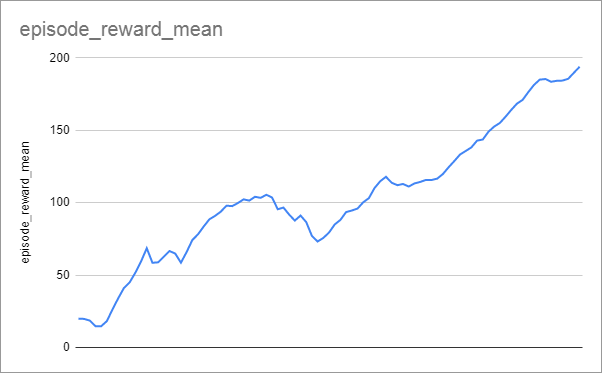
For my run, learning progress (episode_reward_mean from progress.csv) looked like this, taking 176 seconds to reach the target reward of 190:

Note that we didn’t change any of the interesting parameters, such as the learning rate. This environment is simple enough that RLlib’s default parameters for the DQN algorithm do a good job without needing any finessing.
Video
The trained agent interacting with its environment looks something like this:

Bullet CartPole Environment With PPO
Changing the Algorithm
A good thing about using RLlib is that switching algorithms is simple. To train using Proximal Policy Optimisation (PPO) instead of DQN, add the following import:
from ray.rllib.agents.ppo import PPOTrainer
and change the definition of TRAINER as follows:
TRAINER = PPOTrainer
We will find out more details about PPO in a later article when we use it for training the Humanoid environment. For now, we just treat it as a black box and use its default learning parameters.
Graph
When I ran this, training took 109.6 seconds and progress looked like this:

Now that’s a lovely smooth graph! And it trained more swiftly, too.
The videos look similar to those from the training session with the DQN algorithm, so I won’t repeat them here.
Continuous CartPole Environment With PPO
Introduction to the Environment
As mentioned before, traditional CartPole has a discrete action space: We train a policy to pick "move left" or "move right."
PyBullet also includes a continuous version of the CartPole environment, where the action specifies a single floating-point value representing the force to apply to the cart (positive for one direction, negative for the other).
>>> import gym
>>> import pybullet_envs
>>> env = gym.make('CartPoleContinuousBulletEnv-v0')
>>> env.observation_space
Box(4,)
>>> env.action_space
Box(1,)
The observation space is the same as before, but this time the action space is continuous instead of discrete.
The DQN algorithm cannot work with continuous action spaces. PPO can, so let’s do it.
Code
Change the declaration of the environment in the training code as follows:
ENV = 'CartPoleContinuousBulletEnv-v0'
Graph
This time the model took 108.6 seconds to train (no significant difference from the discrete environment), and progress looked like this:

Video
The resulting video looks like this:

There’s more oscillation happening, but it has learned to balance the pole.
Next time
In the next article, we will take a look at two of the simpler locomotion environments that PyBullet makes available and train agents to solve them.
This member has not yet provided a Biography. Assume it's interesting and varied, and probably something to do with programming.


