COVID-19 Diagnosis Using ResNet50 Transfer Learning: Building a DL Network from Scratch

• Download source - 300.4 KB

In this series of articles, we’ll apply a Deep Learning (DL) network, ResNet50, to diagnose Covid-19 in chest X-ray images. We’ll use Python’s TensorFlow library to train the neural network on a Jupyter Notebook.

The tools and libraries you’ll need for this project are:

IDE:

• Jupyter Notebook

Libraries:

• TensorFlow 2.0
• Keras
• NumPy
• Matplotlib
• CV2

We are assuming that you are familiar with deep learning with Python and Jupyter notebooks. If you're new to Python, start with this tutorial. And if you aren't yet familiar with Jupyter, start here.

In the previous articles of this series, we used a transfer learning-based approach to fine-tune an existing ResNet50 model to diagnose COVID-19. In this article, we’ll show you how to build a network from scratch and then train it to classify chest X-ray images into COVID-19 and Normal.

Install Libraries and Load Dataset

We’ll use only TensorFlow, Keras, and OS, along with some basic additional libraries, to build our network for diagnosing COVID-19.

# Import required libraries
import tensorflow as tf
from keras import optimizers
import os, shutil
import matplotlib.pyplot as plt

First, let’s load the data that will be used to train and test the network. In this case, we’ll use a different loading technique from the one we’ve used for the transfer learning-based network. We’ll use the same dataset though.

base_dir = r'C:\Users\abdul\Desktop\ContentLab\P1\archive\COVID-19 Radiography Database’
train_dir = os.path.join(base_dir, 'train')
test_dir = os.path.join(base_dir, 'test')
train_COV19_dir = os.path.join(train_dir, 'COV19')
train_Normal_dir = os.path.join(train_dir, 'Normal')
test_VOV19_dir = os.path.join(test_dir, 'COV19')
test_Normal_dir = os.path.join(test_dir, 'Normal')

Now, let's print the numbers of the COVID-19 and Normal images in our training and testing sets.

print('total training COV19 images:', len(os.listdir(train_COV19_dir)))
print('total training Normal images:', len(os.listdir(train_Normal_dir)))

print('total test COV19 images:', len(os.listdir(test_VOV19_dir)))
print('total test Normal images:', len(os.listdir(test_Normal_dir)))

The output will be as follows:

Preprocess Data

Before feeding data to the network, images must be preprocessed. For our network-to-be-built, we’ll choose the input format of 128x128x3. All images will be rescaled to this size, which is relatively small — less computation cost. Batch size and class mode need to be set now, for ImageDataGenerator to use.

from keras.preprocessing.image import ImageDataGenerator
train_datagen = ImageDataGenerator(rescale=1./255)
test_datagen = ImageDataGenerator(rescale=1./255)

train_generator = train_datagen.flow_from_directory(train_dir, target_size=(128, 128), batch_size=5, class_mode='categorical')
test_generator = test_datagen.flow_from_directory(test_dir, target_size=(128, 128), batch_size=5, class_mode='categorical')

To check the data and label batch shape, we will use:

for data_batch, labels_batch in train_generator:
    print('data batch shape:', data_batch.shape)
    print('labels batch shape:', labels_batch.shape)
    break

Note that a sequential model expects an input of 4 dimensions (Batch size, X, Y, Channels). This is why the batch should be set before building your network; otherwise, an error will occur.

Build DL Network

A Keras model uses the sequential class to create layers. This is a functional model class that represents a stack of layers. It can be easily imported from Keras.

For our model, we’ll use two layers of Convolution, two of MaxPooling, three of ReLU, one Flatten, and two Dense layers (fully connected). We need to import all the required layers from Keras models such as Conv2D, MaxPooling, and Dense.

from tensorflow.keras.models import Sequential
from tensorflow.keras.layers import Dense, Flatten
from tensorflow.keras.layers import Conv2D
from tensorflow.keras.layers import MaxPooling2D
from tensorflow.keras import backend as k
input_shape=(128, 128, 3)
model = Sequential()
model.add(Conv2D(32, kernel_size=(5, 5), strides=(1, 1),
                 activation='relu',
                 input_shape=input_shape))
model.add(MaxPooling2D(pool_size=(2, 2), strides=(2, 2)))
model.add(Conv2D(64, (5, 5), activation='relu'))
model.add(MaxPooling2D(pool_size=(2, 2)))
model.add(Flatten())
model.add(Dense(512, activation='relu'))
model.add(Dense(2, activation='softmax'))

model.summary()

As you can see above, a convolution layer is called using the Conv2D function, which has three main parameters:

• Filters: sets the number of filters generated in a convolution layer
• Kernel size: the size of the filter, or kernel, used in convolution (must be an odd number)
• Strides: a 2-tuple of integers that defines how the convolution will go along the X and Y axes of the input image

The pooling layer also defines stride (to go through all images) and pool _size, which is the size of the pooling filter, or kernel, used to apply pooling over the input image.

Finally, we can visualize our network:

model.summary()

Train the Network

To train our freshly built network, we need to specify the loss function and optimizer. For this network, we’ll use binary Cross-Entropy, as our target is to classify chest X-rays into two classes: Covid-19 and Normal. We’ll use Stochastic Gradient Descent as an optimizer.

In optimization functions, we need to set the learning rate. This is an important parameter. If it is set too low, the learning process may be longer because the weights will encounter small updates. On the contrary, if it is set too high, the network may overfit. It is preferable to start training our network by setting a low value of learning rate, then gradually increase it while monitoring the network performance.

In this, let's select the learning rate of 0.001.

from keras import optimizers
model.compile(loss='categorical_crossentropy',
optimizer=optimizers.adam(lr=1e-4),
metrics=['acc'])

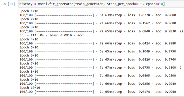
Then, we can start training with 10 epochs (figure 11):

history = model.fit_generator(train_generator, steps_per_epoch=100, epochs=10)

Network accuracy and loss during training can then be plotted using:

acc = history.history['acc']
loss = history.history['loss']
plt.figure()
plt.plot(acc, label='Training Accuracy')
plt.ylabel('Accuracy')
plt.title('Training Accuracy')
plt.figure()
plt.plot(loss, label='Training Loss')
plt.ylabel('Loss')
plt.title('Training Loss')
plt.xlabel('epoch')
plt.show()

Evaluate the Network

As discussed in the previous article, the model can be tested for accuracy on new, unseen images of COVID-19 and Normal classes. In this section, Network was tested on 895 images of COVID-19 and Normal chest X-rays. We used the same testing command used in the previous pre-trained network’s testing "model.evaluate". As seen in figure 10, the network achieved a testing accuracy of 98.8% (figure 13).

Testresults = model.evaluate(test_generator)
print("test loss, test acc:", Testresults)

Next Steps?

We’ve reached the end of our series. We have achieved our set goal which was to classify chest x-rays images into either COVID-19 or Normal. Our employed models achieved well in diagnosing COVID-19 as they reached high testing accuracies of 95% and 98.8% for the transfer learning based model and the newly built model, respectively.

Although our COVID-19 classifier works well, there's still room to improve it. A key addition would be to do additional training to help the network better distinguish COVID-19 from other chest diseases such as viral pneumonia, bacterial pneumonia, mass etc.