Building a Mobile Style Transfer CycleGAN with Keras

• Download project code - 7.2 MB

Introduction

In this series of articles, we’ll present a Mobile Image-to-Image Translation system based on a Cycle-Consistent Adversarial Networks (CycleGAN). We’ll build a CycleGAN that can perform unpaired image-to-image translation, as well as show you some entertaining yet academically deep examples. We’ll also discuss how such a trained network, built with TensorFlow and Keras, can be converted to TensorFlow Lite and used as an app on mobile devices.

We assume that you are familiar with the concepts of Deep Learning, as well as with Jupyter Notebooks and TensorFlow. You are welcome to download the project code.

In the previous article, we discussed the CycleGAN architecture. Now we are done with theory. In this article, we’ll implement the CycleGAN from scratch.

Our CycleGAN will perform unpaired image-to-image translation using the horse-to-zebra dataset, which you can download. We’ll implement our network using TensorFlow and Keras, with the generators and discriminators from the Pix.Pix library. We’ll import the generator and the discriminator via the tensorflow_examples package to simplify the implementation. However, in one of the subsequent articles, we’ll also show you how to build new generators and discriminators from scratch.

It is important to mention that CycleGAN is a very power- and memory-consuming network. Your system must have sufficient RAM of at least 8 GB and a good GPU as good as or better than the GTX 1660 Ti to train and run the CycleGAN with no out-of-memory errors or timeouts.

We’ll train our network using GoogleColab, a hosted Jupyter Notebook service that provides free access to computing resources, including GPUs. Most importantly, it is free, unlike some other cloud computing services.

Processing the Dataset

Let’s load the dataset and apply some preprocessing techniques such as cropping, jittering, and mirroring, which will help us avoid overfitting of the network:

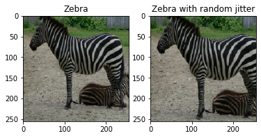
• Image jittering resizes the image to 286 by 286 pixels and then crops it to 256 by 256 pixels from a randomly selected origin point
• Image mirroring flips the image horizontally, from left to right.

The above techniques are described in the original CycleGAN paper.

We’ll upload our data to Google Drive to make it accessible to Google Colab. After the data is uploaded, we can start reading the data. Alternatively, you can simply use tfds.load in your code to directly load the dataset from the TensorFlow datasets package, as we will do below.

First, let’s import some required dependencies:

import tensorflow as tf
import tensorflow_datasets as tfds
from tensorflow_examples.models.pix2pix import pix2pix

import os
import time
import matplotlib.pyplot as plt
from IPython.display import clear_output

AUTOTUNE = tf.data.AUTOTUNE

Now we’ll download the dataset and apply to it the augmentation techniques discussed above:

dataset, metadata = tfds.load('cycle_gan/horse2zebra',
                              with_info=True, as_supervised=True)

train_horses, train_zebras = dataset['trainA'], dataset['trainB']
test_horses, test_zebras = dataset['testA'], dataset['testB']

With the data loaded, let’s add some preprocessing functions:

def random_crop(image):
  cropped_image = tf.image.random_crop(
      image, size=[IMG_HEIGHT, IMG_WIDTH, 3])

  return cropped_image

# normalizing images to [-1, 1]
def normalize(image):
  image = tf.cast(image, tf.float32)
  image = (image / 127.5) - 1
  return image

def random_jitter(image):
  # resizing to 286 x 286 x 3
  image = tf.image.resize(image, [286, 286],
                          method=tf.image.ResizeMethod.NEAREST_NEIGHBOR)

  # randomly cropping to 256 x 256 x 3
  image = random_crop(image)

  # randomly mirroring
  image = tf.image.random_flip_left_right(image)

  return image

def preprocess_image_train(image, label):
  image = random_jitter(image)
  image = normalize(image)
  return image

def preprocess_image_test(image, label):
  image = normalize(image)
  return image

And now, we’ll read the images:

train_horses = train_horses.map(
    preprocess_image_train, num_parallel_calls=AUTOTUNE).cache().shuffle(
    BUFFER_SIZE).batch(1)

train_zebras = train_zebras.map(
    preprocess_image_train, num_parallel_calls=AUTOTUNE).cache().shuffle(
    BUFFER_SIZE).batch(1)

test_horses = test_horses.map(
    preprocess_image_test, num_parallel_calls=AUTOTUNE).cache().shuffle(
    BUFFER_SIZE).batch(1)

test_zebras = test_zebras.map(
    preprocess_image_test, num_parallel_calls=AUTOTUNE).cache().shuffle(
    BUFFER_SIZE).batch(1)

sample_horse = next(iter(train_horses))
sample_zebra = next(iter(train_zebras))
############################Mirroring and jittering
plt.subplot(121)
plt.title('Horse')
plt.imshow(sample_horse[0] * 0.5 + 0.5)

plt.subplot(122)
plt.title('Horse with random mirroring')
plt.imshow(random_jitter(sample_horse[0]) * 0.5 + 0.5)

plt.subplot(121)
plt.title('Zebra')
plt.imshow(sample_horse[0] * 0.5 + 0.5)

plt.subplot(122)
plt.title('Zebra with random jitter')
plt.imshow(random_jitter(sample_horse[0]) * 0.5 + 0.5)

Here is an example of a jittered image.

Building Generators and Discriminators

Now, we import the generators and discriminators from the pix2pix models. We’ll use a U-Net-based generator instead of the residual block one used in the CycleGAN paper. We will use U-Net as it has a less complex structure and requires less computations than a Residual block. However, we will discover the residual block based generator in another article.

OUTPUT_CHANNELS = 3

generator_g = pix2pix.unet_generator(OUTPUT_CHANNELS, norm_type='instancenorm')
generator_f = pix2pix.unet_generator(OUTPUT_CHANNELS, norm_type='instancenorm')

discriminator_x = pix2pix.discriminator(norm_type='instancenorm', target=False)
discriminator_y = pix2pix.discriminator(norm_type='instancenorm', target=False)

With the generators and discriminators in place, we can start setting the losses. Since CycleGAN is an unpaired image-to-image translation, there is no need for paired data to train the network on. Therefore, no one can guarantee that the input and the target images make a meaningful pair during training. That’s why it is important to calculate the cycle-consistency loss to make the network map correctly:

LAMBDA = 10
loss_obj = tf.keras.losses.BinaryCrossentropy(from_logits=True)

def discriminator_loss(real, generated):
  real_loss = loss_obj(tf.ones_like(real), real)

  generated_loss = loss_obj(tf.zeros_like(generated), generated)

  total_disc_loss = real_loss + generated_loss

  return total_disc_loss * 0.5

def generator_loss(generated):
  return loss_obj(tf.ones_like(generated), generated)

Now, we calculate the cycle consistency loss to make sure the translation results are close to the original images:

def calc_cycle_loss(real_image, cycled_image):
  loss1 = tf.reduce_mean(tf.abs(real_image - cycled_image))
  
  return LAMBDA * loss1

def identity_loss(real_image, same_image):
  loss = tf.reduce_mean(tf.abs(real_image - same_image))
  return LAMBDA * 0.5 * loss

Finally, we set optimizers for both generators and discriminators:

generator_g_optimizer = tf.keras.optimizers.Adam(2e-4, beta_1=0.5)
generator_f_optimizer = tf.keras.optimizers.Adam(2e-4, beta_1=0.5)

discriminator_x_optimizer = tf.keras.optimizers.Adam(2e-4, beta_1=0.5)
discriminator_y_optimizer = tf.keras.optimizers.Adam(2e-4, beta_1=0.5)

Next Steps

In the next article, we’ll show you how to train our CycleGAN to translate horses to zebras and zebras to horses. Stay tuned!