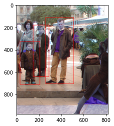
Here we will discuss the challenges we face when dealing with custom object recognition. We’ll also look into algorithms that can help us meet these challenges and implement R-CNN to detect humans in given images.
When working with an object detection algorithm, the basic approach is to try to locate the object of interest by drawing a bounding box around it. Since there could be multiple objects of interest and their number of occurrences are not known beforehand, this results in a variable length output layer, which means the object detection problem cannot be solved by building a standard deep neural network consisting of fully connected layers. One workaround to this problem could be to take different regions of interest from the image and use a neural network to detect the presence of the desired object within each specific region. This approach seems to fail as well since the desired objects could have different aspect ratios and locations within the image resulting in a massive number of regions and eventually computationally blowing up.
To solve the problem, algorithms like R-CNN, Fast R-CNN, and YOLO have been developed. In this article, we’ll implement R-CNN to detect humans in a given image.
R-CNN
Regions with CNN (R-CNN) was introduced by Ross, Jeff and Jitendra in 2014. The idea was that instead of running detection on a huge number of regions, we pass the image through selective search to extract just 2000 regions from the image called region proposals. Now, we can just work with these 2000 proposed regions instead of trying to classify a huge number of regions. Next, we calculate intersection over union (IOU) on proposed regions and add labels using ground truth data. To make sense of everything, we’re going to implement R-CNN from scratch using Keras here, but we’ll definitely get into more details of R-CNN later in the series.
Preparing the Dataset for Object Detection
We’re going to use INRIAPerson dataset which is easily available on kaggle. The mentioned dataset has 2 subdirectories containing Test and Train data and both subdirectories have images along with their associated annotations. Image annotations basically label the data on images and make the objects perceptible to AI and ML models. These images may contain humans, vehicles, or any other type of objects to make it recognizable for machines. However, the INRIAPerson dataset is specifically created to detect persons in the image file and thus only contains annotations for person. Taking a look at the following file will make the idea clear.
="1.0"
<annotation>
<folder>VOC2007</folder>
<filename>crop_000010.png</filename>
<source>
<database>PASperson Database</database>
<annotation>PASperson</annotation>
</source>
<size>
<width>594</width>
<height>720</height>
<depth>3</depth>
</size>
<segmented>0</segmented>
<object>
<name>person</name>
<pose>Unspecified</pose>
<truncated>0</truncated>
<difficult>0</difficult>
<bndbox>
<xmin>194</xmin>
<ymin>127</ymin>
<xmax>413</xmax>
<ymax>647</ymax>
</bndbox>
</object>
</annotation>
We will use these annotations to make the objects recognizable to our model. But before we move forward, we first need to parse these annotations to csv files and extract the data that we need. Python provides the ElementTree API for parsing xml files. Below is a function that can be used to load and parse xml annotation files easily.
def parse_xml_to_csv(path):
xml_list = []
for xml_annot in glob.glob(path + '/*.xml'):
tree = ET.parse(xml_annot)
doc = etree.parse(xml_annot)
count = doc.xpath("count(//object)")
root = tree.getroot()
with open(str(xml_annot)[0:-4]+".csv","w+") as file:
file.write(str(int(count)))
for person in root.findall('object'):
value = (
person[4][0].text,
person[4][1].text,
person[4][2].text,
person[4][3].text
)
coors = " ".join(value)
with open(str(xml_annot)[0:-4]+".csv","a") as file:
file.write("\n")
file.write(coors)
Call the above function, passing the path to annotations files as the argument:
annot_path ="./Annotations"
xml_df = parse_xml_to_csv(annot_path)
Once the function finishes, you can see all the converted csv files.
Implementing R-CNN Using Keras
With our data in place, we can move forward with implementing R-CNN. First, let’s import all the libraries we’re going to work with.
import os
import cv2
import keras
import numpy as np
import pandas as pd
import tensorflow as tf
import matplotlib.pyplot as plt
As we mentioned earlier, searching for regions of interest is computationally exhausting so we will try to implement an efficient solution here. Selective search computes the similarity based on color, texture, size, or shape and hierarchically groups the most similar regions. This process is continued until the whole image becomes a single region. OpenCV offers to implement selective search using the createSelectiveSearchSegmentation function. Add the optimization and selective search to your solution as follows:
cv2.setUseOptimized(True);
selective_search = cv2.ximgproc.segmentation.createSelectiveSearchSegmentation()
Now if we apply selective search on a test image, it would result in bounding boxes around the desired object.

At this point, we’re interested in how accurate our bounding boxes currently are. For that, we can simply use intersection over union (IOU), which is an evaluation metric that measures the accuracy of object detectors. It can be calculated by computing the area of overlap (area of intersection) between the predicted bounding box and the ground-truth bounding box divided by the total area bounded by both (area of union):
def compute_iou(box1, box2):
   x_left = max(box1['x1'], box2['x1'])
   y_top = max(box1['y1'], box2['y1'])
   x_right = min(box1['x2'], box2['x2'])
   y_bottom = min(box1['y2'], box2['y2'])

   intersection_area = (x_right - x_left) * (y_bottom - y_top)

   box1_area = (box1['x2'] - box1['x1']) * (box1['y2'] - box1['y1'])
   box2_area = (box2['x2'] - box2['x1']) * (box2['y2'] - box2['y1'])

   union_area = box1_area + box2_area - intersection_area

   iou = intersection_area / union_area

   return iou
Now we need to pre-process the data to create a dataset that can be passed to our model. We will iterate over all the images and set them as the base for selective search. We’ll then iterate over the first 2000 proposed regions resulting from selective search and calculate the IOU so we can annotate the region of our desired object (a human). The images will be labeled based on the presence of the object and will be appended to our training_images array.
training_images=[]
training_labels=[]
for e,i in enumerate(os.listdir(annot)):
try:
filename = i.split(".")[0]+".png"
img = cv2.imread(os.path.join(path,filename))
dataframe = pd.read_csv(os.path.join(annot,i))
ground_truth_values=[]
for row in dataframe.iterrows():
x1 = int(row[1][0].split(" ")[0])
y1 = int(row[1][0].split(" ")[1])
x2 = int(row[1][0].split(" ")[2])
y2 = int(row[1][0].split(" ")[3])
ground_truth_values.append({"x1":x1,"x2":x2,"y1":y1,"y2":y2})
selective_search.setBaseImage(img)
selective_search.switchToSelectiveSearchFast()
ssresults = selective_search.process()
imout = img.copy()
counter = 0
f_counter = 0
flag = 0
fflag = 0
bflag = 0
for e,result in enumerate(ssresults):
if e < 2000 and flag == 0:
for val in ground_truth_values:
x,y,w,h = result
iou = compute_iou(val,{"x1":x,"x2":x+w,"y1":y,"y2":y+h})
if counter < 20:
if iou > 0.70:
image = imout[y:y+h,x:x+w]
resized = cv2.resize(image, (224,224), interpolation = cv2.INTER_AREA)
training_images.append(resized)
training_labels.append(1)
counter += 1
else :
fflag =1
if f_counter <20:
if iou < 0.3:
image = imout[y:y+h,x:x+w]
resized = cv2.resizetimage, (224,224), interpolation = cv2.INTER_AREA)
training_images.append(resized)
training_labels.append(0)
f_counter += 1
else :
bflag = 1
if fflag == 1 and bflag == 1:
flag = 1
except Exception as e:
print(e)
continue
Now training_images and training_labels contain the new x and y coordinates for our model. Let’s start with the imports for our model.
from keras.layers import Dense
from keras import Model
from keras import optimizers
from keras.optimizers import Adam
from keras.applications.vgg16 import VGG16
from keras.preprocessing.image import ImageDataGenerator
from keras.callbacks import ModelCheckpoint, EarlyStopping
The R-CNN model can technically be fit from scratch, but it costs too much time and results in poor performance. Here, we’ll use transfer learning to save us time and achieve better performance. You can use imagenet or coco weights for transfer learning as per your preference.
vggmodel = VGG16(weights='imagenet', include_top=True)
vggmodel.summary()
The above code fragment results in the following output:

Next, we’ll freeze the first ten layers of the model by setting trainable to false.
for layers in (vggmodel.layers)[:10]:
layers.trainable = False
We’re only interested in the presence or non-presence of humans, which means we have only two classes to predict, so we’ll add two unit dense layers with softmax activation. The reason for using softmax activation is that it ensures the sum of outputs is 1 (that is, the outputs are probabilities).
X= vggmodel.layers[-2].output
predictions = Dense(2, activation="softmax")(X)
Finally, we’ll use Adam optimizer to compile the model.
model_final = Model(vggmodel.input, predictions)
model_final.compile(loss = keras.losses.categorical_crossentropy, optimizer = Adam(lr=0.001), metrics=["accuracy"])
We’ve created our model. Before moving forward, we need to encode the dataset. We can use LabelBinarizer for encoding.
class Label_Binarizer(LabelBinarizer):
	def transform(self, y_old):
    	Y = super().transform(y_old)
    	if self.y_type_ == 'binary':
        	return np.hstack((Y, 1-Y))
    	else:
    	    return Y
	def inverse(self, Y):
    	if self.y_type_ == 'binary':
        	return super().inverse(Y[:, 0])
    	else:
        	return super().inverse(Y)
encoded = Label_Binarizer()
Y =  encoded.fit_transform(y_new)
We also need to split our dataset into training and test sets which can be done using train_test_split from sklearn. Here we're splitting the data into an 80% training, 20% testing ratio.
X_train, X_test , y_train, y_test = train_test_split(X_new,Y,test_size=0.20)
Keras provides ImageDataGenerator to pass the dataset to the model. You can also apply horizontal or vertical flips to increase the dataset.
train_data_prep = ImageDataGenerator(horizontal_flip=True, vertical_flip=True, rotation_range=90)
trainingdata = train_data_prep.flow(x=X_train, y=y_train)
test_data_prep = ImageDataGenerator(horizontal_flip=True, vertical_flip=True, rotation_range=90)
testingdata = test_data_prep.flow(x=X_test, y=y_test)
Adding Keras Callbacks
Training deep neural networks takes a lot of time and we’re always at a risk of wasting computational resources. To avoid this problem, Keras offers two callbacks: EarlyStopping and ModelCheckPoint. EarlyStopping is called when an epoch finishes. It aborts the training process once it no longer improves, allowing you to configure any number of epochs. ModelCheckpoint is also called after every epoch and saves the best performing model automatically. We can use both callbacks when training our model using fit_generator as follows:
checkpoint = ModelCheckpoint("rcnn.h5", monitor='val_loss', verbose=1, save_best_only=True, save_weights_only=False, mode='auto', save_freq=1)
early = EarlyStopping(monitor='val_loss', min_delta=0, patience=100, verbose=1, mode='auto')
hist = model_final.fit_generator(generator= traindata, steps_per_epoch= 10, epochs= 500, validation_data= testdata, validation_steps=2, callbacks=[checkpoint,early])
Testing Our Model
Our model will now be created and saved as rcnn.h5 and we’re in a good position to get predictions on our model. We’ll follow the same steps as before: Iterate over all images and set them as base images for selective search. Later, we’ll pass selective search results to our model for prediction, and our model will create bounding boxes when it encounters a human in the image.
count=0
for e,i in enumerate(os.listdir(path)):

	count += 1
	image = cv2.imread(os.path.join(path,i))
	selective_search.setBaseImage(image)
    selective_search.switchToSelectiveSearchFast()
	ssresults = selective_search.process()
	imout = image.copy()
	for e, res in enumerate(ssresults):
    	if e < 2000:
        	x,y,w,h = res
        	test_image = imout[y:y+h,x:x+w]
        	resized = cv2.resize(test_image, (224,224), interpolation = cv2.INTER_AREA)
        	image = np.expand_dims(resized, axis=0)
        	out= model_final.predict(image)
        	if out[0][0] > 0.65:
            	cv2.rectangle(imout, (x, y), (x+w, y+h), (0, 255, 0), 1, cv2.LINE_AA)
	plt.figure()
	plt.imshow(imout)


Note: Results are from an early termination
Limitations of R-CNN
R-CNN comes along with some drawbacks. It still implements the sliding window at its root. The only difference is that it is actually implemented as a convolution which makes it more efficient than traditional sliding window techniques. But it still needs to run a full forward pass of CNN for each of the 2000 region proposals and has a complex multi-stage training pipeline, resulting in big performance concerns. Also, because of high testing time, R-CNN becomes infeasible in real time or congested areas.
What’s next?
In this article, we learned to implement our first custom object detector using deep neural networks in Keras. We also discussed some limitations of the approach. In the next article of the series, we will try to overcome the limitations imposed by R-CNN and will also get an estimate of the number of people present in an area.
C# Corner MVP, UGRAD alumni, student, programmer and an author.
 General
  News
News  Suggestion
  Question
  Bug
Bug  Answer
  Joke
Joke  Praise
  Rant
Rant  Admin
Admin 


